Can we learn functions, not weights? Yes we KAN!
[Paper: KAN: Kolmogorov-Arnold Networks]
Summary by Adrian Wilkins-Caruana
What is a neural network? An archetype is a multilayer perceptron (MLP). MLPs are probably the most widely used architectural component of the NN variants we’re familiar with, like transformers and CNNs. But have you ever considered why this is the case? What if there was something else — maybe even something better — that we could use instead of MLPs? Today’s summary explores a new kind of NN building block called Kolmogorov-Arnold Networks, or KANs. As we’ll see, KANs are a fascinating new way to think about and construct NNs, and they may also offer some insight into why MLPs are so ubiquitous in today’s NN models.
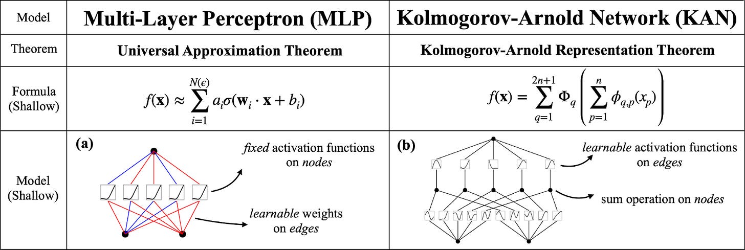
According to Liu et al., KANs were inspired by the Kolmogorov-Arnold Representation Theorem, a mathematical theorem that says it’s possible to write a complicated, multivariate function using a bunch of simpler, univariate ones. If this sounds familiar, that’s because it’s very similar to the universal approximation theorem that underpins MLPs! MLPs work by combining input signals with learnable weights and a fixed activation function, and KANs work by combining inputs with learnable activation functions. The network representations in the figure below show this distinction. We can see that the MLP has different weights (indicated by the red and blue edges) and a fixed activation function (in this case, SiLU), whereas the KAN has much more complex edges that are summed together.
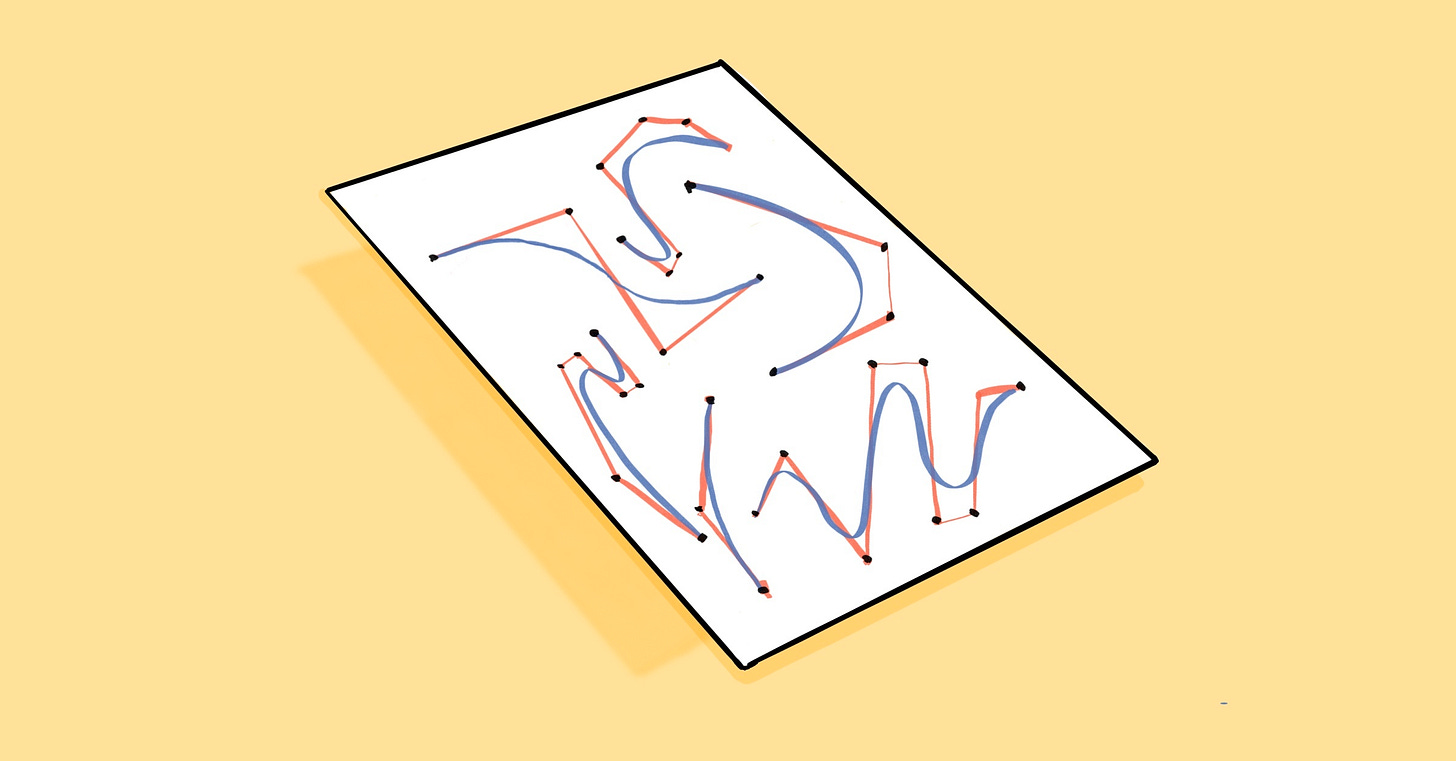
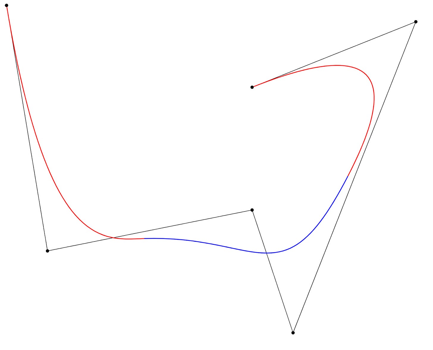
In a KAN, the activation functions are special piecewise functions called B-splines. If you’ve ever used the Bezier curve tool in Adobe Photoshop or a similar tool, then you might already have an intuitive idea about how B-splines can model an arbitrary function. The figure below shows a curve that is a weighted sum of several B-splines. The shape of the splines (and thus the overall curve) is controlled by the position of the anchor points. During training, the positions of these points are optimized so that the resulting splines act as useful activation functions.
Using splines as the basis of the “neurons” in a KAN yields an NN with useful properties. For starters, KANs are more interpretable than MLPs, since visual representations of their complex activations are much more understandable than reading the raw weights of an MLP layer. Additionally, more parameters can be added to a KAN after partial training to improve its accuracy (after more training to improve the added parameters). Unlike MLPs — where added parameters can affect the whole NN — each additional KAN parameter only affects two splines (if the splines are quadratic), leaving the other splines unaffected. To use another Photoshop analogy, this is like drawing a rough outline of an object with a small number of Bezier curves, and then adding in more points later to refine it.
Another benefit is that sometimes a simpler KAN can be better than a more complex one. For example, the researchers used two different KANs to fit a two-parameter function. To describe these networks, they used the notation [n_0, n_1, …, n_L], where n_0 is the number of inputs or parameters in the data, n_i is the number of nodes or activation functions in layer i, and L is the total number of layers. For a certain two-parameter function, the authors tried a [2, 5, 1] KAN and a [2, 1, 1] KAN. The figure below shows the expression for the function f(x,y) that the KAN is fitting, and the error levels (RMSE) over training time. You can see that the [2, 1, 1] KAN achieves a lower test/training loss overall at the marked interpolation threshold.
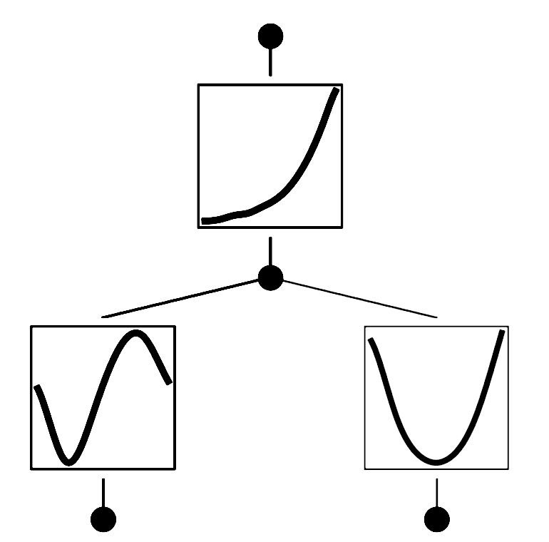
The reason for the stepped nature of the loss in these training results is that, during training, the researchers progressively added more splines to each of the KAN’s activation functions, improving their accuracy. This is indicated by the “grid” information printed on the plots. It makes intuitive sense that the [2, 1, 1] KAN should perform better since it only takes two activations to fit the data in this case: one that sums a spline each for sin(πx) and y^2, and another for exp. The figure below shows what the activation functions would look like in this [2, 1, 1] KAN.
Unfortunately, this paper only demonstrates the ability of KANs on toy datasets like the one above. They didn’t run tests on a simple real-world dataset, like the MNIST dataset. One reason for this might be because training a KAN is about 10x slower than training an MLP with the same number of parameters — though this may just be due to an inefficient training implementation that could improve as more researchers iterate on the training algorithm.
Also, while KANs seem to offer several advantages compared to MLPs, they are limited in several ways. For example, a KAN’s activation is only defined on a fixed set of input values, since splines don’t extend infinitely across the input’s domain. And, while KANs may be interpretable in toy examples, I’m not convinced that being able to observe the activations in a more complex KAN — say, one with more than a dozen layers — would really be that helpful. And of course there’s the argument that MLPs are already universal approximators, so an MLP can also represent a KAN. So I won’t hold my breath waiting for KANs to revolutionize NNs. But they’re cool nonetheless, and they may have some niche mathematical applications, such as for symbolic regression or knot theory. If that sounds interesting to you, then I highly recommend you give this paper a read!


