A neural network that makes neural networks
[Paper: Neural Network Diffusion]
Summary by Adrian Wilkins-Caruana
By now, you've probably heard of diffusion models. They’re those neural networks that transform an array of useless values, like random noise, into an array of meaningful data. Diffusion models are most famous for generating images and videos that — you guessed it — are arrays of useful data. You know what else are just arrays of useful data? Neural network parameters! So, can diffusion models be used to turn noise into useful network parameters? That’s the question that Wang et al. try to answer in their recent paper: Neural Network Diffusion.
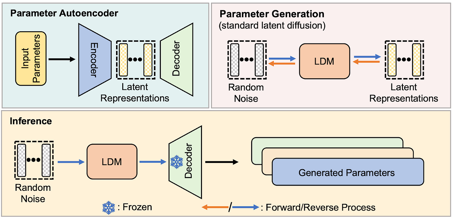
How is it even possible to diffuse the parameters of a neural network (NN)? Architecturally, the setup is pretty much identical to how diffusion models generate images or video. The authors (Wang et al.) call their method p-diff (for “parameter diffusion”).The setup, shown in the figure below, involves a parameter autoencoder (upper left) and a latent diffusion model a.k.a. LDM (upper right). Once the autoencoder is trained (more on this later), its decoder can be used to generate network parameters from the diffused latent representations (lower half).
Instead of training on web-scale datasets of images and video, the researchers compiled their own datasets of neural network parameters. Each dataset consists of very minor variations to a subset of a single NN’s parameters. To acquire these parameter variations, the researchers trained a model from scratch, and then — in the last epoch of training — froze the non-subset weights and continued to train the subset of weights that the diffusion model will be able to generate. Checkpoints of the subset weights slowly changed during this final period of training, and these are what the researchers used to train the LDM and autoencoder.
Training then proceeded as normal: First, the autoencoder was trained to encode latent representations of the input parameters, and the decoder had to decode them to recreate the input parameters by minimizing the mean-squared reconstruction error. Then, the LDM was trained to remove noise from noisy latent representations of the input parameters from the dataset. This all means that this trained autoencoder and LDM can only diffuse parameters for a single model, not several different models.
You might be wondering, “Are the different variations of parameter subsets really diverse enough to train p-diff to generate distinct representations? Essentially, is p-diff just memorizing the input data?” One way to check would be to compare how well the model with diffused parameters performs on tests compared to regularly trained models. Unsurprisingly, models with diffused parameters perform better when there are more parameter variants in its training set. But, given enough training data, models with diffused parameters perform about on par with their regularly trained counterparts, not reliably better.
That doesn’t really answer our question though. Maybe p-diff has just learned to copy the parameters of the model that performs best in its training data. The authors wondered this too, so they devised a similarity metric to compare two different models. The method compares the agreement between the two models’ predictions: It’s 100% when they precisely agree on the classification for examples in a test dataset, and 0% when they disagree on every example (and in between for partial agreement).
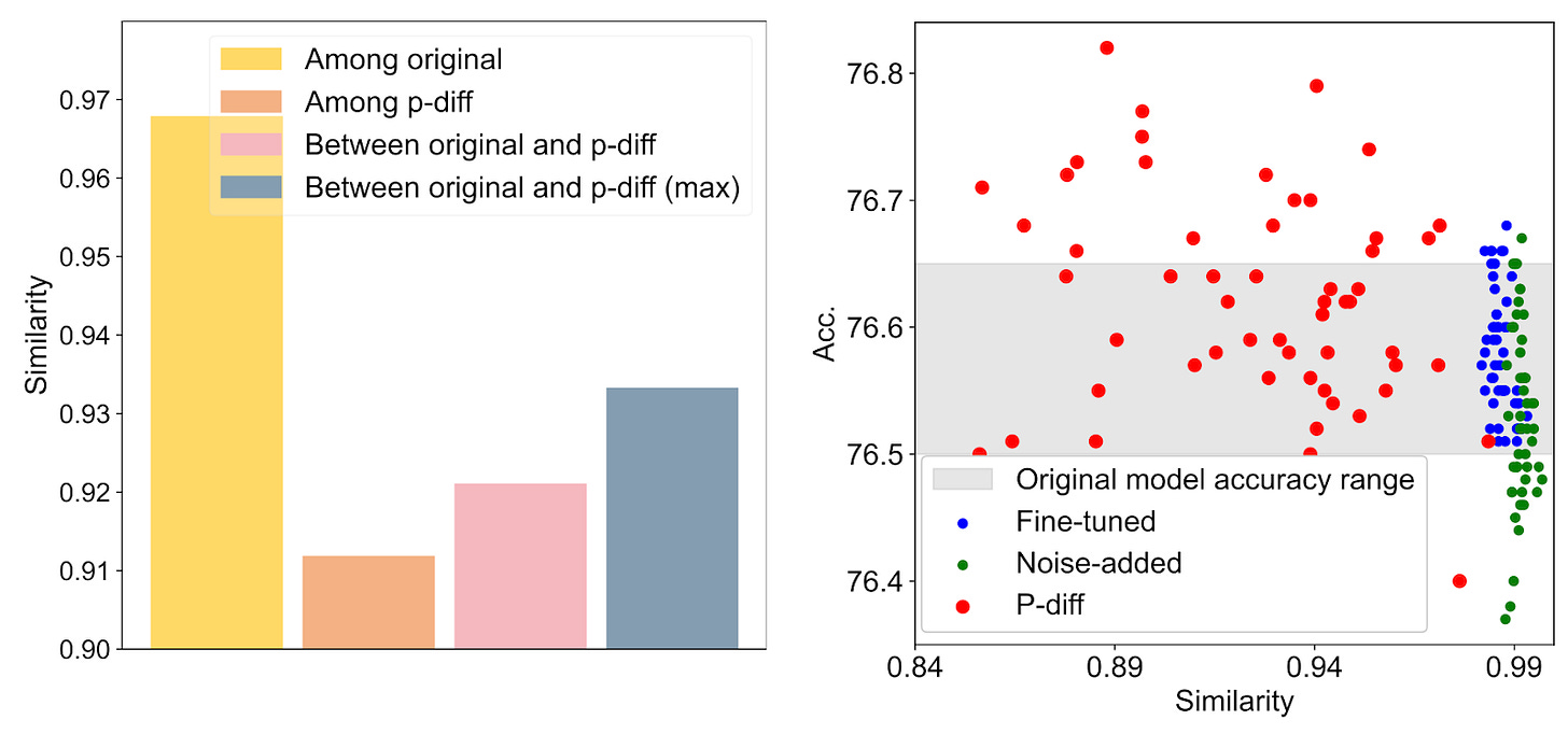
The figure below compares original models with p-diff models. In the bar chart, the mean similarity among original models (yellow) is much higher than the mean similarity among p-diff models (orange); yet the similarity among pairs of original-to-p-diff models is a little bit higher than p-diff models alone (pink). This indicates that p-diff models are more distinct from each other than from original models, but not by much.
The upper scatter plot compares the accuracy of individual models from the bar chart (y-axis) with their similarity to a single baseline model (x-axis). Original models (blue) all achieve similar accuracy and are very similar to each other, while p-diff models perform differently, sometimes much better or worse. Finally, the lower scatter plot shows a t-SNE plot of the models’ parameters. Since the p-diff points and original points are in their own clusters, the takeaway is that there’s something distinct about each set of parameters (since t-SNE can distinguish between them), but it’s not entirely clear what, as t-SNE is a bit of a black-box.
In my opinion, I don’t see methods like p-diff being used for practical applications any time soon — NNs are already a black-box, and applying a subsequent NN that changes the original’s parameters in a non-obvious way seems a bit dubious. But, as a research exercise, p-diff is absolutely fascinating! I’ve always imagined a NN’s parameters and its inputs pairing as being very tightly yet delicately coupled to each other and, aside from further training, changes to some or all of the parameters would throw the whole NN out of whack. But with p-diff, that isn’t the case at all. I’d love to see future research delve deeper into what the differences are between p-diff models and vanilla ones — that would help me understand what p-diff learns from the parameter subsets in its training data.


